Final Report
Last updated March 16th, 2026
Video Summary
Summary
Space Invaders is a classic fixed-shooter game where the player controls a starfighter, attacking and dodging enemies from above. Rather than treating this as a one-off application, our project uses Space Invaders as a controlled testbed for comparing and understanding reinforcement learning (RL) methods.
To make broad comparisons feasible, we will primarily use MinAtar SpaceInvaders through Gymnasium. MinAtar provides a simplified 10×10, channel-based observation space that trains much faster than full Atari, enabling us to run multiple seeds, hyperparameter sweeps, and component ablations within our compute budget. If time permits, we will validate key findings on the full ALE Space Invaders environment.zs
Approach
DQN
Deep Q-Network(DQN) is a model-free, value-based reinforcement learning algorithm. DQN is a popular method for training video games, and performs well when there are a large number of states. DQN is based on Q-Learning, which is a model free algorithm that iteratively tests states and actions using rewards from a table of Q-Values. Q-Learning struggles with large numbers of states and continuous actions, so Deep Q-Learning replaces this table in Q-Learning with a neural network that approximates Q-Values. The input to this network is the state, it outputs Q-values for all possible actions.
Loss function: \(\mathcal{L}_\theta = (r + \gamma \max_{a'} Q_{\bar{\theta}}(s', a') - Q_\theta(s, a))^2\)
In the MinAtar environment, the agent receives a reward of +1 for every opponent destroyed, and there are no negative rewards. The agent uses a discrete action space with 6 possible outputs corresponding to moving and shooting. The MinAtar environment suffers from partial observability, where the agent cannot interpret the direction of a moving object since it is shown in a static frame. To combat this problem we used temporal frame stacking, where groups of four frames are stacked together to give more context about the direction of the moving object. Frame stacking provided improved performance of the agent, as it could determine whether bullets were moving at it or away from it.
We chose to train the Stable-Baselines3 DQN implementation. We first trained DQN without adjusting any hyperparameters on runs of 100,000, 500,000, and 1,000,000 timesteps, comparing the results of using temporal frame stacking to the results without it. To continue, we added similar hyperparameters to the MinAtar paper(Young, Tian, 2019), and tuned them iteratively on runs of 1,000,000 timesteps. Some significant hyperparameters that we tuned were the exploration fraction, learning rate, and target update interval.
QRDQN
The next algorithm we chose to investigate was Quantile Regression Deep Q-Network(QRDQN), as a version was available on Stable-Baselines3-contrib library which kept consistent with our baseline DQN implementation. QRDQN is a distributional reinforcement learning algorithm that builds on top of DQN by using quantile regression to parametrize the return distribution, rather than estimating a single scalar mean. QR-DQN modifies the output layer of standard DQN to produce N quantile values per action, which helps account for uncertainty in the environment. Since it tracks the full distribution, the distributional approach helps avoid the overestimation problem that is a known weakness of DQN.
Loss function: Quantile Huber Loss for a specific quantile τ:
\[\rho_\tau^\kappa(u) = |\tau - \delta_{\{u < 0\}}| \mathcal{L}_\kappa(u)\]The QRDQN implementation used the same reward, action space and time step trials were used along with 4 frame temporal stacking. Again, we started evaluating no hyperparameters with and without temporal frame stacking. The same hyperparameter set as the DQN implementation was used to avoid changing too many variables, and to focus on comparing the algorithms themselves.
Rainbow DQN
Rainbow DQN is a model-free, value-based reinforcement learning algorithm that extends the base DQN by combining six improvements into a single agent: Double DQN, Dueling Networks, Prioritized Experience Replay, Multi-step Returns, Distributional RL (C51), and Noisy Networks. Rainbow is a popular method for training video game agents and performs well in environments with large state spaces. Rather than introducing a fundamentally new algorithm, Rainbow demonstrates that these six components are complementary and jointly produce significantly better performance than any individual enhancement alone.
The core extension over standard DQN is the distributional approach to Q-learning, where instead of estimating a single expected Q-value per action, the network learns a full probability distribution over returns. Noisy Networks replace the standard ε-greedy exploration strategy with learnable parametric noise in the network weights, and the Dueling architecture separates the value and advantage streams to improve Q-value estimation. Double DQN reduces overestimation bias by using the online network to select actions and the target network to evaluate them.
Loss function:
\[\mathcal{L}(\theta) = -\frac{1}{B}\sum_{i=1}^{B} w_i \sum_z m(z) \log p_\theta(z \mid s_i, a_i)\]We applied Rainbow DQN to the MinAtar Space Invaders environment, training for 5,000,000 frames. The reward structure grants +1 for each enemy destroyed with no penalties, and the agent operates over a discrete action space of 6 moves corresponding to directional movement and shooting. Unlike standard DQN which uses a uniform replay buffer, Rainbow leverages a prioritized replay buffer of size 100,000 that samples transitions proportionally to their loss magnitude, controlled by a priority exponent of α = 0.5. This ensures the agent learns more frequently from surprising or high error experiences. Rather than bootstrapping from a single next step, 3-step returns are used to propagate reward signals further back through time, improving credit assignment. The important sampling exponent β is gradually annealed from 0.4 to 1.0 throughout training to correct for the sampling bias introduced by prioritization. The target network is synchronized with the online network via a hard update every 1,000 gradient steps, and all parameters are optimized using Adam with a learning rate of 1×10⁻⁴.
PPO
For this project, we implemented the Proximal Policy Optimization (PPO) algorithm to train an agent in the MinAtar Space Invaders environment. We chose PPO because it is generally more stable and easier to tune than other policy gradient methods. The core of our approach relies on an Actor-Critic architecture that optimizes a “clipped” surrogate objective. This objective prevents the policy from changing too drastically in a single update, which helps keep the training stable.
Following the work of Schulman et al. (2017), the loss function we optimized is:
\[L^{CLIP}(\theta) = \mathbb{E}_t\left[\min\left(r_t(\theta)\hat{A}_t,\ \text{clip}(r_t(\theta), 1-\epsilon, 1+\epsilon)\hat{A}_t\right)\right]\] \[\hat{A}_t^{GAE(\gamma,\lambda)} = \sum_{l=0}^{\infty}(\gamma\lambda)^l\delta_{t+l}\]where rt(θ) is the probability ratio between the new and old policies, and ε is the clipping hyperparameter (set to 0.2 in the baseline). To estimate the advantage Ât, we used Generalized Advantage Estimation (GAE), which was introduced by Schulman et al. (2015) to balance bias and variance in policy gradients.
Here, δ represents the TD error, γ is the discount factor (0.99), and λ is the smoothing parameter (0.95). These settings helped the agent learn a more consistent value function in the discrete 10×10 grid of MinAtar.
Regarding the scenario setup, the state input consists of the 10×10 game grid. However, since a single frame does not show the direction of moving bullets, we used Frame Stacking (k=4) to give the agent a sense of motion. The action space is discrete, allowing the agent to move and fire. For the training process, we ran the model for roughly 200,000 iterations, totaling over 100 million interaction steps to ensure full convergence.
To study how different design choices affect PPO training behavior, we evaluated several experimental configurations. Starting from a baseline implementation, we tested variations involving different learning schedules, reward formulations, and architectural adjustments. These configurations were trained under the same environment and interaction budget to ensure a fair comparison. The resulting training curves provide insight into the learning dynamics of PPO across these configurations and are analyzed in the following evaluation section.
Evaluation
DQN
To evaluate the performance our DQN agent, we conducted a series of test trials across 20 independent games for each training configuration(baseline, frame stacking, frame stacking and tuned hyperparameters). We recorded the maximum, minimum, and mean scores, alongside the average survival time which is an important metric in a game like Space Invaders. We also tested a random policy to serve as a baseline to compare our agent performance to.
Analyzing these metrics we learned that the frame stacking nearly doubled the average score compared to the baseline policy, and the final version with the hyperparameters tuned scored significantly higher than that. More importantly, the agent demonstrated a significant increase in survival time, incorporating more defense and dodging with the hyperparameters.
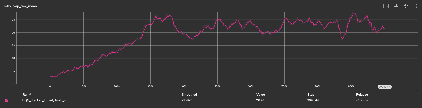
The learning curve shown from the final training we ran for the mean episode reward (ep_rew_mean) shows a linear increase within the first 300,000 timesteps followed by a more steady refinement of the policy through 1 million steps, which is influenced by our choice of the exploration fraction. This plateau may indicate that the agent had finished learning, and could possibly be trained on less timesteps that 1 million, increasing efficiency.
The DQN agent with tuned hyperparameters and temporal frame stacking significantly outperformed the versions without hyperparameters and frame stacking as expected, and is used to evaluate the other advanced methods against.
| Version | Timesteps | Avg Score | Avg Survival(frames) | Key behavior |
|---|---|---|---|---|
| Random Policy | N/A | 2.5 | 50 | n/a |
| Baseline | 1M | 14.2 | 110 | Static firing. |
| Stacked | 1M | 26.5 | 195 | Active dodging, predicts bullet paths. |
| Stacked + Tuned | 1M | 42.95 | 324 | Left, right, fire, right+fire, more variety of actions |
QRDQN
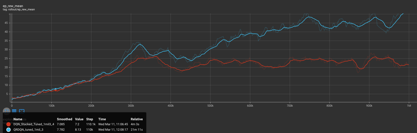
When comparing the QRDQN average metrics from the 1,000,000 timestep trained agent across 20 games to the top DQN version, we observe that QRDQN significantly outperforms the average score and survival time. The learning curve shown in the graph is interesting, as we see the QRDQN on pace with DQN, but when DQN starts to plateau QRDQN continues to learn and ends with a higher performance. Evaluating the results, we can conclude that QRDQN learning the full distribution of potential rewards helps the agent perform better in fast moving and complex environments like Space Invaders, compared to DQN estimating a single expected average.
| Version | Timesteps | Avg Score | Avg Survival(frames) | Key Behavior |
|---|---|---|---|---|
| Random Policy | n/a | 2.5 | 50 | n/a |
| DQN | 1M | 42.95 | 324 | Left, right, fire, right+fire |
| QRDQN | 1M | 76.5 | 588 | Left, right, fire, left+fire, dodged bullets better, more accurate |
Rainbow DQN
To evaluate the performance of our Rainbow DQN agent, we tested 20 independent games at four training checkpoints (250k, 500k, 750k, and 1M frames), recording the score and survival length for each. We also tracked the training evaluation mean over the full 5,000,000-frame training run to observe long-term learning dynamics.
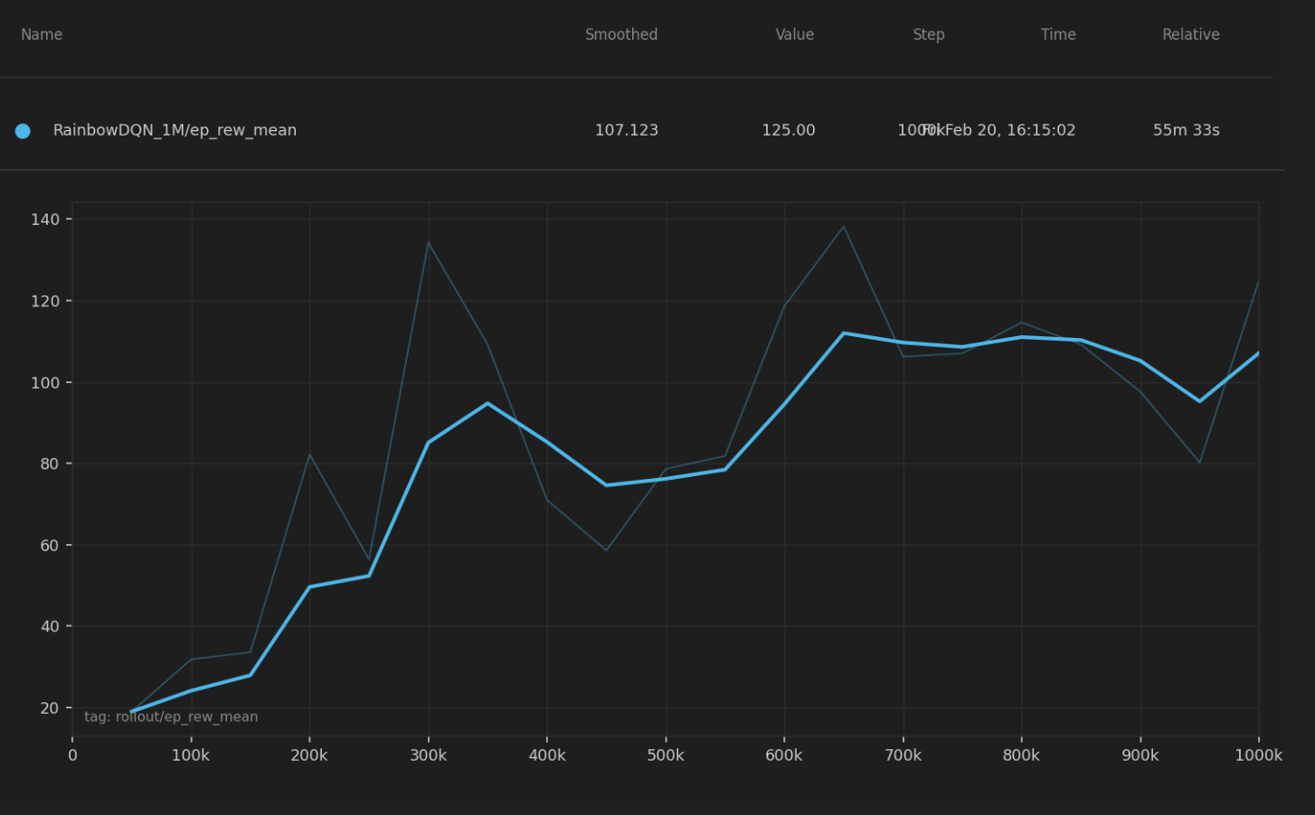
At the 1M frame checkpoint, the agent averaged a score of 106.0 and a survival time of 818 frames across 20 games, already surpassing the best DQN performance. Notably, the agent exhibited high variance. Some episodes produced scores as high as 237 while others ended quickly with scores near 22, suggesting the agent had learned strong strategies in favorable configurations but remained sensitive to early-game difficulty. This bimodal behavior is characteristic of distributional methods, where the agent models the full return distribution and can commit aggressively to high-value action sequences.
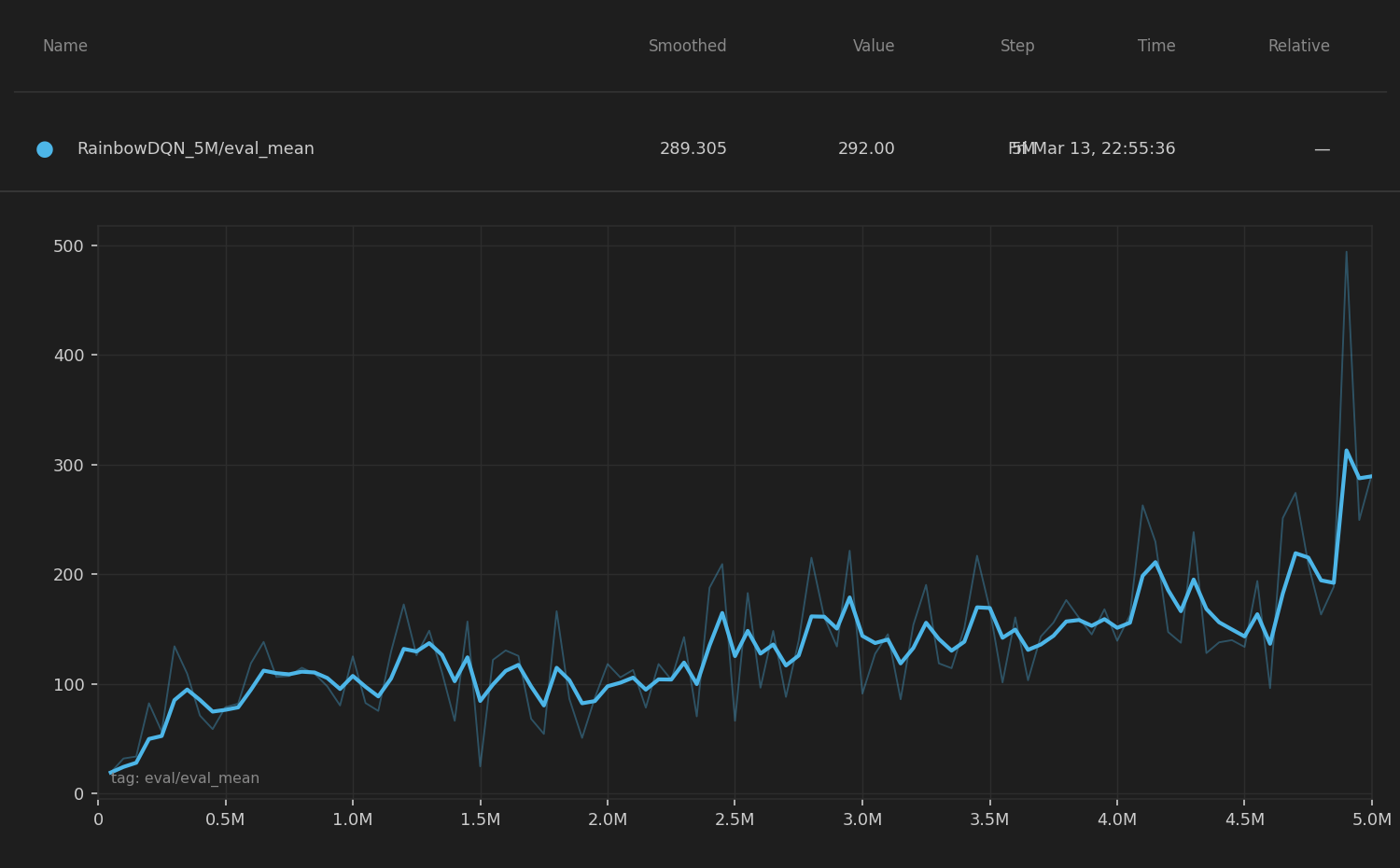
The learning curve over the full 5M frame run shows a clear upward trend, with eval mean rising steeply in the first 1M frames and continuing to improve gradually thereafter. By 5M frames, the agent reached an evaluation mean of 292.0, demonstrating that Rainbow benefits significantly from extended training compared to DQN and QRDQN. The continuous improvement without a clear plateau suggests the distributional and noisy network components help the agent keep refining its policy rather than converging prematurely.
Comparing Rainbow DQN to DQN and QRDQN at the 1M frame mark, Rainbow already outperforms DQN by a large margin. Its full 5M-frame performance far exceeds both prior methods, confirming that the combination of distributional RL, prioritized replay, multi-step returns, and noisy exploration produces substantially better agents in the stochastic, fast-moving MinAtar Space Invaders environment.
| Version | Steps | Avg Score | Max Score | Min Score | Avg Survival | Key Behavior |
|---|---|---|---|---|---|---|
| Rainbow | 250k | 74.8 | 167.0 | 7.0 | 635.9 frames | Right+Fire 58%, Left 21%, Fire 18% |
| Rainbow | 500k | 79.6 | 166.0 | 18.0 | 596.6 frames | Right+Fire 56%, Left 20%, Fire 18% |
| Rainbow | 750k | 94.0 | 236.0 | 7.0 | 693.0 frames | Right+Fire 48%, Left 21%, Fire 19% |
| Rainbow | 1M | 106.0 | 237.0 | 22.0 | 817.8 frames | Right+Fire 42%, Left 19%, Fire 17% |
| Version | Frames | Avg Score | Avg Survival (frames) | Key Behavior |
|---|---|---|---|---|
| Rainbow DQN | 1M | 106.0 | 818 | High variance, aggressive play, strong when alive |
| Rainbow DQN | 5M | ~292.0 | — | Sustained improvement, highly refined policy |
In this section, we evaluate our PPO implementation through two main experiments: training dynamics across multiple configurations and a component-level ablation study.
PPO Training Dynamics
Unlike the final cross-algorithm comparison, this PPO analysis focuses on the training dynamics within the MinAtar 10×10 environment. Therefore, the x-axis is expressed in training iterations, which more clearly illustrates policy updates and protocol adjustments during development.
Quantitative Results
To better contextualize these learning curves, Table 1 summarizes the key hyperparameters used in each experimental configuration:
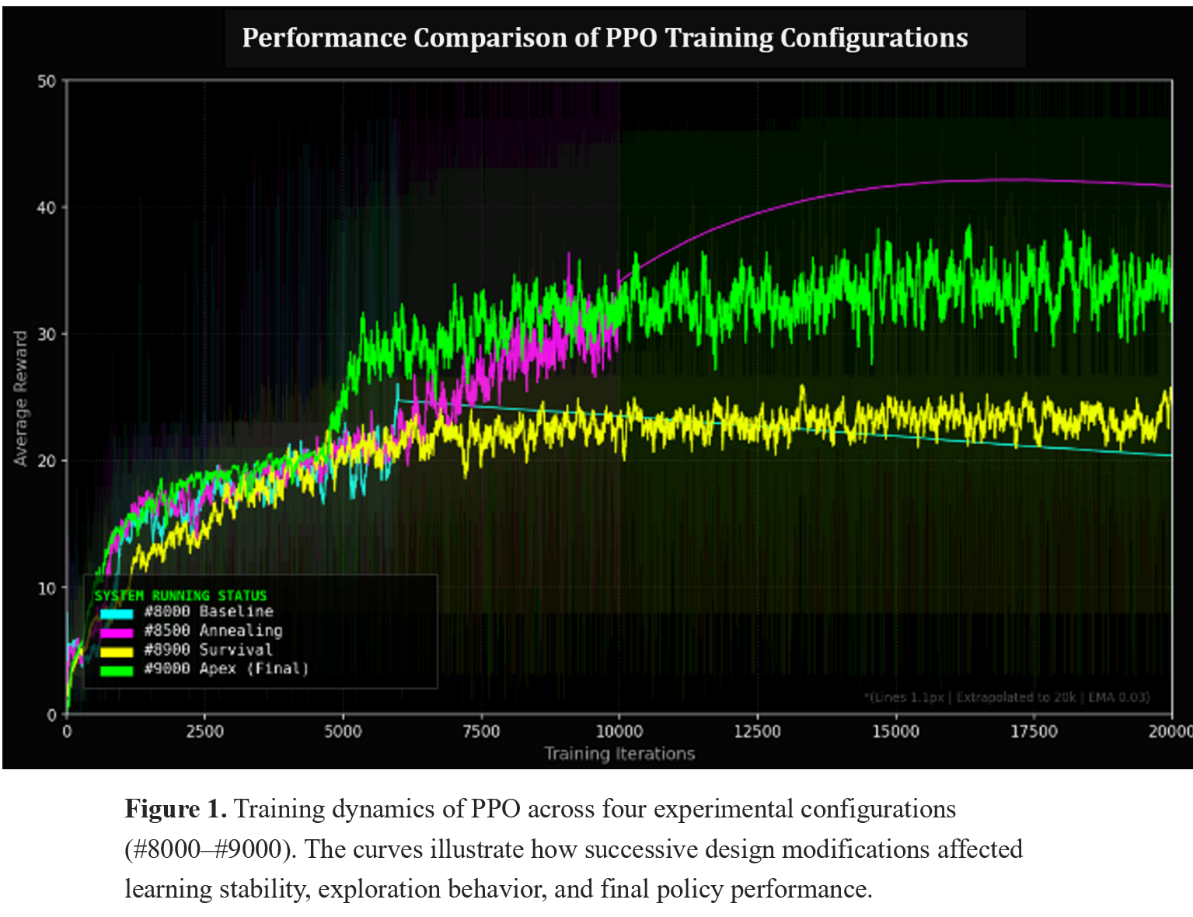
Table 1. PPO Experimental Configurations and Performance Summary for Figure 1
| Exp ID | Protocol | Iterations | LR Schedule | Entropy / Regularization | Architecture & Environment | Result (Peak / Mean) & Diagnosis |
|---|---|---|---|---|---|---|
| #8000 | Baseline (Dual Decay) | 10,000 | Linear decay 3e-4 → 5e-5 | Entropy decay 0.01 → 0.001 | Pure environment rewards; standard initialization; 1 action per frame | Peak: 213.0 / Mean: 56.98 — High potential but unstable late-stage variance |
| #8500 | OpenAI Protocol | 10,000 | Linear decay to zero | Clip annealing → 0 | Strict mimicry of long-horizon Atari parameters | Peak: 118.0 / Mean: 35.54 — Early convergence; exploration suppressed |
| #8900 | Genesis (Reward Shaping) | 20,000 | 2.5e-4 → 1e-5 | Fixed entropy = 0.01 | Ortho-init + Frame Skip (4×) + Survival bonus | Peak: 46.4 / Mean: 24.25 — Survival trap; policy plateau |
| #9000 | Apex (DNA Repaired) | 20,000 | Pure #8000 decay | Pure #8000 decay | Ortho-init + Frame Skip (4×); no survival bonus | Peak: 61.0 / Mean: 33.51 — Micro-control failure in 10×10 grid |
Qualitative Results
The PPO agent was developed through an iterative optimization process. The baseline PPO (cyan line) initially improved but quickly showed early convergence, indicating limited exploration. To accelerate learning, an annealing protocol (magenta line) was introduced, but the agent soon experienced training stagnation, suggesting that the aggressive decay restricted further policy improvement. To address early deaths in the environment, a survival incentive (yellow line) was added, which increased episode length but led to a survival trap, where the agent prioritized staying alive over scoring. Finally, the Apex protocol (green line) removed the survival bias and restored a balanced reward structure, producing the most stable and higher-performing policy. This iterative process allowed the PPO agent to progressively diagnose and correct training behaviors, ultimately leading to a robust final configuration.
PPO Component Ablation Study
To better understand the contribution of individual components in our PPO implementation, we conducted an ablation study by systematically removing several key elements from the baseline configuration.
Quantitative Results
To provide clarity on the experimental setup, the specific hyperparameter modifications used in each ablation configuration are summarized in Table 2.
Table 2. PPO Component Ablation Design and Observed Learning Effects
| Curve | Configuration | Component Removed | Key Setting | Observed Effect |
|---|---|---|---|---|
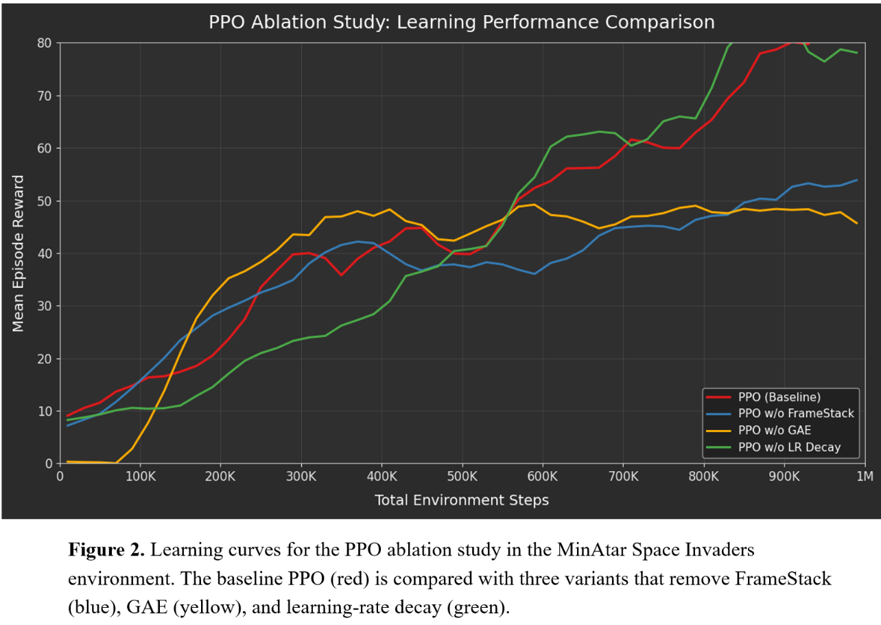
| 🔴 | PPO-Full (Baseline) | None | GAE (λ = 0.95), FrameStack (k = 4), Linear LR Decay | Stable learning progression and highest final reward. Provides balanced variance reduction and temporal perception. |
| 🔵 | PPO w/o FrameStack | Temporal Context | FrameStack removed (k = 1) | Performance consistently lower. Lack of temporal information limits the agent’s ability to infer invader motion, leading to reduced policy quality. |
| 🟡 | PPO w/o GAE | Advantage Estimation | GAE disabled (λ = 0, equivalent to 1-step TD) | Fast early improvement but clear performance plateau. High variance in advantage estimates disrupts stable policy optimization. |
| 🟢 | PPO w/o LR Decay | Optimization Scheduling | Constant learning rate (no decay) | Higher peak rewards but increased oscillation. Absence of decay leads to less stable convergence during later training stages. |
Qualitative Results
To understand the contribution of key components in PPO, we conducted an ablation study where one component was removed at a time while keeping the rest of the training setup unchanged. Figure 2 compares the baseline PPO with three variants: without FrameStack, without GAE, and without learning-rate decay. The baseline model shows the most stable learning curve and achieves the highest mean episode reward.
Removing FrameStack slows down learning because the agent only observes a single frame and cannot easily infer motion in the environment. Removing GAE leads to faster initial learning but quickly reaches a performance plateau, suggesting that noisy advantage estimates make policy updates less stable. Without learning-rate decay, the training curve shows larger fluctuations. Overall, the results indicate that all components contribute to PPO’s learning dynamics, with GAE playing a particularly important role in stabilizing policy optimization.
Final Performance Comparison Across Algorithms
To summarize the overall outcomes of our experiments, we compare the final performance of the four reinforcement learning algorithms evaluated in this project.
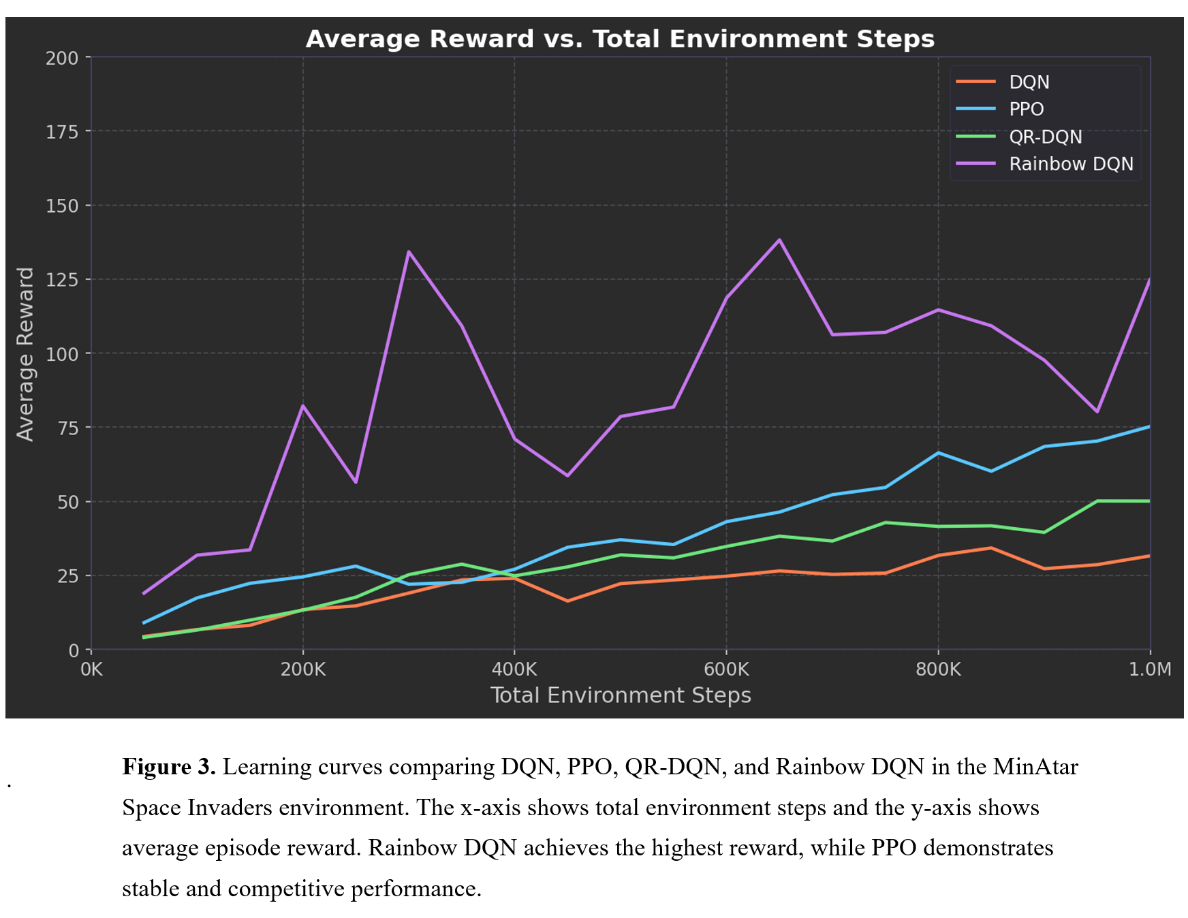
Table 3. Final performance comparison of PPO, DQN, QRDQN and Rainbow DQN in the MinAtar Space Invaders environment.
| Algorithm | Final Avg Reward | Learning Stability | Sample Efficiency | Key Idea |
|---|---|---|---|---|
| DQN | 32 | Medium | Medium | Value-based Q-learning |
| QR-DQN | 50 | Medium–High | High | Distributional Q-learning |
| Rainbow DQN | 125 | High but unstable spikes | Very High | Multi-technique DQN variant |
| PPO | 73 | High | Medium | Policy-gradient with Actor–Critic |
Conclusion
This study compared policy-gradient methods (PPO) with value-based methods from the DQN family to understand how different reinforcement learning paradigms solve the same task in the MinAtar Space Invaders environment. The results show clear differences between the algorithms. Rainbow DQN achieves the highest reward, benefiting from improvements such as prioritized replay and distributional learning. QR-DQN also outperforms the original DQN, suggesting that modeling value distributions improves learning effectiveness. PPO performs competitively and demonstrates stable learning behavior, although its final reward remains lower than the strongest DQN variants.
Overall, the results highlight an important trade-off between learning stability and performance efficiency. As noted by John Schulman et al. (2017), policy-gradient methods such as PPO emphasize stable policy updates and exploration, which can lead to steadier learning curves. However, in small discrete environments like MinAtar Space Invaders, value-based methods often achieve higher scores. Consistent with observations reported in De La Fuente et al. (2024), our results suggest that in reinforcement learning there is rarely a single algorithm that performs best across all tasks.
Resources Used
Reinforcement Learning Libraries
- PyTorch — used to implement the PPO neural network, policy updates, and training pipeline.
- NumPy — used for numerical operations during training and data processing.
- Stable Baselines3 and Stable Baselines3 Contrib - used their DQN and QRDQN algorithms.
Environment and Benchmark
- MinAtar Environment (Young & Tian, 2019) — used as the experimental environment for the Space Invaders task.
- OpenAI Gym-style interface — used to interact with the environment and run training episodes.
Development Tools
- Python 3.13
- Visual Studio Code — used for implementing, debugging, and running PPO experiments.
- Matplotlib — used to generate training curves and comparison plots.
Algorithm References
- Schulman et al., 2017 (PPO Paper) — main reference for implementing the clipped PPO objective.
- Schulman et al., 2015 (GAE) — reference for implementing Generalized Advantage Estimation.
- Young & Tian, 2019 (MinAtar paper) - reference for DQN starting hyperparameters.
Online Documentation
- PyTorch Documentation
- MinAtar GitHub Repository
- OpenAI Gym Documentation
- Stable Baselines3 and Stable Baselines3 Contrib Documentation
Data Visualization Tools
- Matplotlib — used to generate reward curves and algorithm comparison figures.
- Python plotting scripts — used to visualize PPO training dynamics and ablation results.
Use of AI Tools
- ChatGPT (OpenAI) was used as a support tool for discussion and clarification of reinforcement learning concepts (e.g., PPO training dynamics and experiment design).
- It was also used for minor editing and language polishing of written explanations in the report.
- ChatGPT was used for coding assistance and debugging with the DQN and QRDQN implementation, testing, and recording.
- Claude Code was used for assisting with the development of the Rainbow DQN.
- AI tools were not used to generate the final PPO implementation, experimental code, or evaluation results.
- All algorithm implementations, experiments, plots, and analysis were written and executed by the author.
References
De La Fuente, N., & Vidal Guerra, D. A. (2024). A comparative study of deep reinforcement learning models: DQN vs PPO vs A2C. arXiv preprint arXiv:2407.14151.
Schulman, J., Wolski, F., Dhariwal, P., Radford, A., & Klimov, O. (2017). Proximal Policy Optimization Algorithms. arXiv preprint arXiv:1707.06347.
Young, K., & Tian, T. (2019). MinAtar: An Atari-Inspired Testbed for Thorough and Reproducible Reinforcement Learning Experiments. arXiv preprint arXiv:1903.03176.
Schwarzer, M., Obando-Ceron, J., Courville, A., Bellemare, M., Agarwal, R., & Castro, P. S. (2023). Bigger, Better, Faster: Human-level Atari with human-level efficiency. arXiv. https://doi.org/10.48550/arXiv.2305.19452
MinAtar Space Invaders - Pgx Documentation
MinAtar Github Repository - https://github.com/kenjyoung/MinAtar
Stable-Baselines3 DQN Documentation — https://stable-baselines3.readthedocs.io/en/master/modules/dqn.html
Stable-Baselines3-contrib QRDQN Documentation— https://sb3-contrib.readthedocs.io/en/master/modules/qrdqn.html
QRDQN arXiv — https://arxiv.org/pdf/1710.10044
QRDQN explained — https://www.emergentmind.com/topics/quantile-regression-deep-q-network-qr-dqn
Playing Atari with Deep Reinforcement Learning 2013 paper — https://arxiv.org/abs/1312.5602
Human-level control through deep reinforcement learning 2015 paper — https://www.nature.com/articles/nature14236